Quantum Physics II — Data collection, modelling, and analysis at CMS CERN

CMS ALGORITHMS FOR ANALYTICS AND DARK MATTER DETECTION
In this second part of the previous introductory article, we’ll tackle the more in-depth description of data collection, object modelling, and data analysis at CMS. The general workflow behind these kinds of experiments is complex, but I’ll try to give a brief description of each part so you can get a general idea of the whole process.
Analysis of a collision and important concepts
We‘ve been talking about particles and detectors, but an important question remains unanswered: what exactly is colliding? The answer is protons, or more exactly, bunches of protons. Accelerated through the LHC by multiple solenoid setups, these bunches come across one another in the detectors, and a collision happens. This proton beam has no perpendicular component, meaning it only moves in a circular manner through the LHC, due to the solenoids’ magnetic field; this is done on purpose since studying the collision in the perpendicular plane means the conservation of energy applies and all momentum must be null, meaning if there’s an imbalance an invisible particle has been produced. A cross-section of the detector can be seen below, with its components (here). Some examples of these particles are neutrinos, but also possible dark matter or other theoretical particles. So now, what’s the next step?

At the interaction vertex, these particles collide and decay products flow through the different parts of the detector, constructed so that measures are taken with high precision and allow for the (mostly) unequivocal identification of particles. However, not everything is as straightforward as it seems, and several events need to be taken into account; I’ll briefly explain them below.
One of the most important magnitudes in colliders is luminosity, which is interpreted as the number of collisions per unit of time and surface. As of 2018, when Run 2 ended, the luminosity value meant that every 25 ns a collision occurred and that almost 150 femtobarns of cumulative data (each femtobarn equals 100 billion collisions!) were analysed.
This raises a significant problem: it’s obvious that more collisions are needed to assess the veracity of models, but if there are too many, the detector won’t be able to keep up with them; this is further complicated since the interactions are among proton bunches. The concept is known as pile-up, and it refers to the average number of collisions that occur each time the detector tries to check the decay products of an interaction. With current data, this value is around 20 collisions, but CERN is allocating its resources to an upgrade called High-Luminosity LHC, which will improve on the integrated luminosity and, in turn, increase the pile-up to almost 200; this is unfeasible with current hardware and software, meaning this project will need serious backing and development; however, the benefits far outweigh the difficulties.
Okay, and now that we know a lot of collisions occur at almost the same time, how is CMS able to discern the decay products of the interaction it wants? Not only that, but the amount of data produced is orders of magnitude over what current hardware and software can process and store. This is the core process of CERN data gathering, and it’s taken care of by several software and hardware solutions commonly referred to as trigger. It’s a really interesting and core part of the data gathering process, but it’s too extensive and technical to discuss here, so I’ll explain the methodology behind it briefly and leave some documentation here, here, and here in case you’re interested. I’ll also leave a diagram below that summarises this information.
The first phase filters down a lot of data using detector hardware to register adequate data in a really short time (almost a millionth of a second!), taking into account information from the muon chambers and calorimeters specifically, and is known as the level-1 trigger or L1. This phase can cut down the total recorded data from 40 MHz up to just 100 kHz, offering the first cut towards useful data. Next, a second set of commercial processors and parallel machines takes that data and further refines it based on precision parameters, operating offline; this is called the high-level trigger or HLT. Then, it creates a backup of the data and sends it to the associated research institutions for analysis. Even at this last stage, recorded data is still around the 1 GB/s mark, showing just how much the trigger and further resources are needed.
Collision object identification
Now that collision data has been recorded, the next step is to identify the particles based on their traces through the detector. This will allow scientists to reconstruct the particles that have appeared as a result of the collision, using the data collected at the different parts of the detector. These reconstructions of particles at CMS employ an algorithm called Particle Flow; the algorithm itself is really complex and takes into account many measurements and variables to discriminate between particles and correctly tag them, so please check the documentation provided if you’re interested.
With this algorithm, photons and leptons (especially muons) are easily tagged with the algorithm, but more complex objects such as hadrons are harder to tag. The difficulty associated with this jet tagging is related to the nature of the Strong force and a concept called sea quarks that we’ll discuss briefly next.
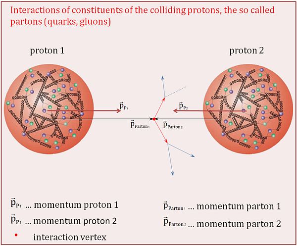
In a collision between two protons, or more accurately between proton quarks, the immediate thought is that only the constituent quarks can interact, so only up and down quarks would interact. However, a measure of the mass of the proton and these quarks shows that most of the mass doesn’t come from its constituents but from internal bounding energy. This means that this excess energy, if the collider energy is enough, can produce other quarks such as quarks bottom and top, both several times the mass of quarks u and d, and these quarks may be the ones that interact at the collision point; an example of a collision may be seen in the image below.
An important concept of jet tagging is that, usually, the decay-inducing quark is unknown since the hadronisation process is so chaotic, but a certain type of jet can be identified. Jets coming from the decay of a b quark have a characteristic second vertex, which has enough travel distance from the first as to be measured (the reason is that b quarks have a longer lifetime than other quarks); for this reason, it’s perceived as a separate important event and receives the name b-tagging. This event has a specific algorithm created to detect it called CVS.
Data simulation and model checking
Once meaningful data has been retrieved and objects are recreated, it’s time to check this data against previously known results for the SM. The way CERN takes care of this comparison is by employing data simulations with MonteCarlo samples. These simulations include all data related to processes’ cross-sections (defined as the probability of decay related to all possible decays), decays, and detector components (to the point of knowing the location of each pixel!) so that the uncertainty of these controllable events is minimised and meaningful conclusions can be made; if we want to measure a cross-section for dark matter, which may be very low, these uncertainties could be either the defining point of discovery or just statistical variations.
The algorithms simulate particles moving through the detector, interacting with each other, showing decay channels to high perturbation theory orders, and in general being very precise with the locations and efficiency of each and every part of the detector. The main algorithms used in this simulation are Powheg and aMC@NLO, both of them built on Pythia. Afterwards, the software Geant4 simulates the particle interactions with the CMS detector. These algorithms provide SM-accurate processes for all the different backgrounds needed in the analysis, which we will explain next.
Now that we have collected real collision data and have data simulations, the next step is to define the process we want to study, like a certain decay of particles producing dark matter. To check if dark matter production is possible in this model, the investigator must include in its data all the possible backgrounds; in this context, a background is a decay that leaves the same traces in the detector as the main process we want to study.
It’s mandatory at this state to include blinding to the data, meaning that we shouldn’t include real data until the end of the study; this prevents the investigator from being biased.
Finally, the goal of these discovery projects can be summarised in one sentence: after including the simulation data, the investigator selects measures like the number of jets, tagged b quarks, missing transverse energy, etc. or defines new ones that they think could potentially be used to discriminate the signal (the studied process) against the backgrounds; this means, for example, selecting variable intervals where the dark matter processes are abundant while background processes are not.
Afterwards, the investigator includes the real data and checks if the results are in agreement with the SM. The way this is done is by a hypothesis test of:
- H0: SM physics
- H1: BSM physics
This includes doing some advanced statistical analysis, like creating a modified likelihood ratio to obtain confidence intervals (CI) of the cross-sections of these processes. This is very technical so I’ll leave some documentation here that hints at the entire process, but the basic idea behind it is that we can compare the obtained results with what is expected and:
- If they’re similar, then the investigator has fine-tuned the limits of the cross-section of the model for future references, and further studies of that model are made easier.
- If they aren’t similar, then they might have discovered something new! In particle physics, this case is presented when differences between theoretical and experimental cross-sections exceed 2𝝈 uncertainty, but it’s not classified as a discovery until the 5𝝈 threshold; 𝝈 in this context refers to the confidence interval associated, and this article gives a really good explanation of this concept. This shows that, in particle physics, we are really certain of the results obtained.
As an example, the most recent case of this 5𝝈 threshold was the discovery of the Higgs boson back in 2012.
Conclusion
The goal of this article is to show the reader the workflow of a CMS investigator researching a certain process, either a search for new particles like dark matter or already studied processes. From the detector components to the data collection, simulation and analysis, I hope you have acquired a general understanding of these concepts, albeit very superficial. In that regard, the literature regarding this subject is written by CERN physicists, so assumptions about all these steps are regularly made, and the average reader will be lost in the concepts and common slang employed.
I hope this article has helped you get a better understanding of this workflow, and that it’ll maybe spark some interest in particle physics, helping you understand further research done and news stories about it.